Neural Networks and Deep Learning

• toproofread
• machine-learning
• course

#course #machine-learning #toproofread

This is the second course of the Coursera Deep Learning Specialisation by Andrew Ng. The notebook index is here.

According to the course description on Coursera:

In the second course of the Deep Learning Specialization, you will open the deep learning black box to understand the processes that drive performance and generate good results systematically.

By the end, you will learn the best practices to train and develop test sets and analyze bias/variance for building deep learning applications; be able to use standard neural network techniques such as initialization, L2 and dropout regularization, hyperparameter tuning, batch normalization, and gradient checking; implement and apply a variety of optimization algorithms, such as mini-batch gradient descent, Momentum, RMSprop and Adam, and check for their convergence; and implement a neural network in TensorFlow.

The Deep Learning Specialization is our foundational program that will help you understand the capabilities, challenges, and consequences of deep learning and prepare you to participate in the development of leading-edge AI technology. It provides a pathway for you to gain the knowledge and skills to apply machine learning to your work, level up your technical career, and take the definitive step in the world of AI.

Objective:

Discover and experiment with a variety of different initialization methods, apply L2 regularization and dropout to avoid model overfitting, then apply gradient checking to identify errors in a fraud detection model.

• Decisions we need to make when implementing
  • Num of layers
  • Hidden units
  • Learning rates
  • Activation functions
• However, we don’t really know what’s best at the beginning, which is why we need to experiment with different choices. It’s an iterative process
• The optimal hyperparameters also depends on the hardware and the field
• Important to consider how fast can your iteration process can be
• Training, development, and testing data
  • What data should be used for training, testing, development, etc.
    • The development set is for evaluating which method is the best
    • The test set is for evaluating the result
    • The old school practice is 70%/30% or 60%/20%/20%
    • However, now we have larger data data set so the new school might use less for development and testing
  • Mismatched train/test distribution
    • This happens when the different sets come from different sources
    • This should therefore be avoided
  • The test is optional because the development set can be used for testing
• Bias and variance
  • There used to be a trade off, but with modern method it matters less
  • We can visualise bias and variance in 2d
    
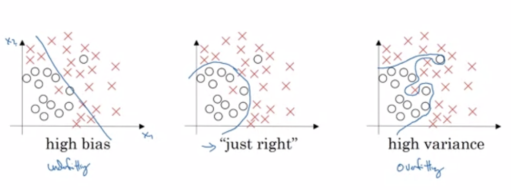
  • Calculation:
    • Assume human error, aka base error, is 0%, but if otherwise, the machine is considered low bias if its error is close to human error
    • High variance when train set error is very different from dev set error as a result of overfitting
    • High bias when the error is high on both sets, meaning that the NN underfits the training set
• Systematic way to improve machine learning
  • If high bias, try:
    • bigger network
    • training longer
    • other NN architecture
  • Elif high variance, try:
    • more data
    • regularisation
    • other NN architecture

• This is a thing we do to prevent overfitting
  • So don’t use when it’s not overfitting
• There are different ways to do it:
  • L1
  • L2 aka weight decay
  • Dropout regularisation
• L2 regularisation
  • To implement this, we add something to the cost function as shown here
    
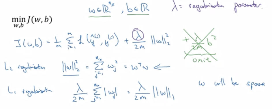
    • The Forbenius norm^[a norm is something like the distance from the origin to the point but in higher dimensions. It can be (maybe) thought of like a higher dimensional absolute value] formula says that $$\left|w^{[l]}\right|^{2}=\sum_{i=1}^{n^{l}} \sum_{j=1}^{n^{[l-1]}}\left(w_{i, j}^{[l]}\right)^{2}$$
  • After doing that, dw becomes: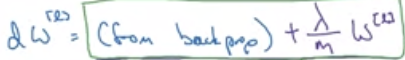
    
  • The intuition can be:
    • the added term to the cost function incentivises the network to make the ws close to zero –> hence reducing the impact of hidden layers –> hence reducing the variance
    • smaller weights makes the pre-squishification output land closer to zero on the activation function –> the network appears closer to linear –> lower variance[^remember that a network all activation functions is effectively linear]
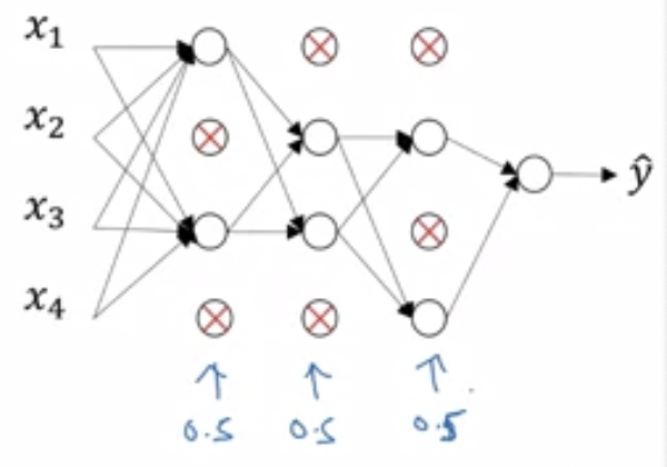
• Dropout regularisation
  • Basically, randomly disable nodes for each training example
    
  • Intuition
    • we are training smaller networks for each example
    • neurons spread out their reliance on each input because they can drop out at any time
  • Implementation (with l=3 as example)
    1. generate a random matrix of zeros and ones by d3 = np.random.rand(a3.shape[0], a3.shape[1]) < 0.8 (the 0.8 is the probability that a number in the matrix will be 1)
    2. Zero out some elements by element wise multiplication a3 = np.multply(a3, d3)
    3. Scale up a3 by doing a3 /= 0.8
  • Choosing keep-prop probability by how big the layer is.
  • Don’t use drop out when testing
  • The cost function will not be well defined because dropout is random
• Data augmentation
  • Flipping training data (for computer vision)
  • Taking random crops or rotations (for computer vision)
  • Add random distortion (for hand writing recognition)
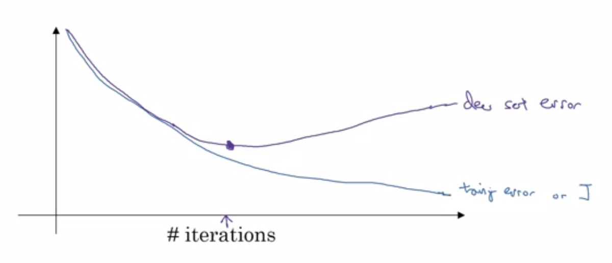
• Early stopping
  • stop there
    
• Orthogonalisation
  • meaning: take care of only one thing at a time

• Normalisation
  • This is when we do this
    
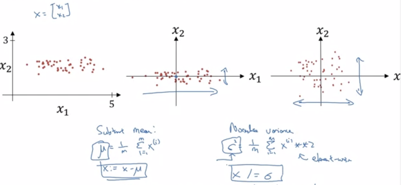
  • Why does this help?
    • It makes gradient descend easier because dramatically different range can make gradient descend go in the wrong direction.
• Vanishing/Exploding gradients
  • in deep networks, weights grow or shrink exponentially with L so they can explode or vanish
  • Solution: smarter weight initialisation
    • We want the variance of the weights for a layer to be small if the layer is big because high variance leads to high activation and thus explosion or vanishing.
    • To do this, we initialise the weights based on the number of neurons in the previous layer according to the equation $\text{Var}(w_i) = \frac{1}{n}$
    • To do this, we can use w = np.random.rand(shape here) * np.sqrt(1/n[l-1])
    • For ReLU, it works better with $\text{Var}(w_i) = \frac{2}{n}$ for some reason
    • The reason why this works has something to do with Gaussian random method
    • For some other reason, according to a paper, tanh works better with $\text{Var}(w_i) = \sqrt{\frac{1}{n}}$
• Gradient checking
  • This helps to check if we did things correctly
  • Numerical approximation of gradients
    • Basically, use two triangles to estimate gradient
      
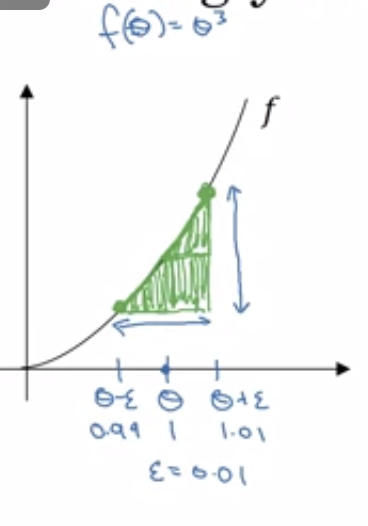
    • This runs slower though
    • The error for using this method turns out to be $O(\epsilon^2)$, so using small $\epsilon^2$ makes the error small
  • Steps
    1. Reshape all weights and biases into vector
    2. Concatenate all vectors $\theta$
    3. Reshape all derivatives of weights and biases into vector
    4. Concat that into another giant vector $d\theta$
    5. Check by approximation and comparison
       
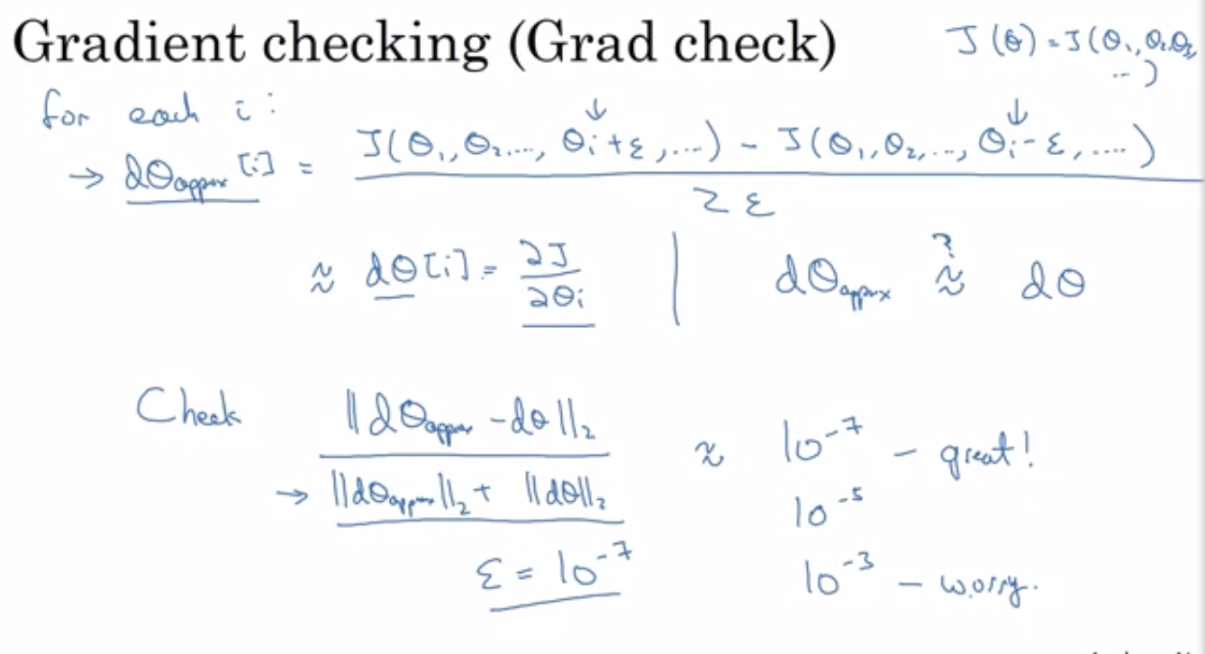
  • Good practices
    • Don’t check when training because it’s slow
    • If gradient check fails, try locate where it fails
    • Remember L2 regularisation
    • Don’t use it for dropout

Objective:

Develop your deep learning toolbox by adding more advanced optimizations, random minibatching, and learning rate decay scheduling to speed up your models.

• This is a way to speed up training by making some gradient descent before going through all training examples.
• Use this when the data set is so large that using all of them at once doesn’t help
• Mini-batch simply beans splitting up big training data into smaller batches
• Notation: we use superscript $^{{t}}$ to indicate the different mini-batches. For example $X^{{34}}$ indicates the 34th batch
• Implementation
  • All we do is process a subset of training example at a time (a function to do this is helpful)
  • Then we loop through all the mini-batches to do the same.
• Mini-batch size
  • size = m is essentially a batch grad descent (use when m <= 2000)
  • size = 1 is called stochastic grad descent and will be very noisy (and it doesn’t make good use of vectorisation)
  • size in between is good (maybe 1000, but $2^n$ is usually more efficient)
  • Trials and errors help as always
  • It has to be small enough for the data to fit in RAM

• When we have noisy data, we can do some kind of average calculation to smooth out the data.
• We usually use a moving average
  • Denoted $v$
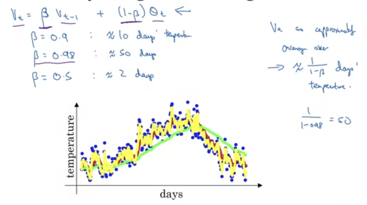
  • The general formula is, for each data point $\theta_t$, $v_t = \beta v_{t-1} + (1 - \beta)\theta_t$.
  • $\frac{1}{1 - \beta}$ is approximately how long the average rolls over. The higher the smoother
    
  • This saves computational resources
  • $\beta = 0.9$ is usually good
• Bias correction
  • Basically, this fixes the average curve starting low (because we set the first point to zero)
  • To fix this, take $\frac{v_t}{1-\beta}$ for the original $v_t$ value which affects mostly the beginning.

• Basically, we average previous derivatives using the moving average method and use the gradient with momentum to do learning.
• This makes gradient descent smoother and usually make learning faster
• Imagine:
  • derivative = acceleration
  • moving average = velocity
• Implementation:
  • For each iteration $t$:
    • Calculate $dW, db$ for current mini-batch
    • $v_{d W}=\beta v_{d W}+(1-\beta) d W$
    • $v_{d b}=\beta v_{d b}+(1-\beta) d b$
    • $W=W-\alpha v_{d W}, \quad b=b-\alpha v_{d b}$
    • (don’t worry about bias correction)

• This is something similar but uses squares and squareroots
• Implementation
  • For each iteration $t$:
    • Calculate $dW, db$ for current mini-batch
    • $S_{d W}=\beta S_{d W}+(1-\beta) d W^{2}$
    • $S_{d b}=\beta S_{d b}+(1-\beta) d b^{2}$
    • $W:=W-\alpha \frac{d W}{\sqrt{s_{d W}} + \epsilon} \quad b:=b-\alpha \frac{d b}{\sqrt{s_{d b}} + \epsilon}$
  • Note:
    • the $\beta$ is another $\beta$
    • the $\epsilon = 10^{-8}$ ensures bottom is not zero

• This is a combination of and
• Implementation
  
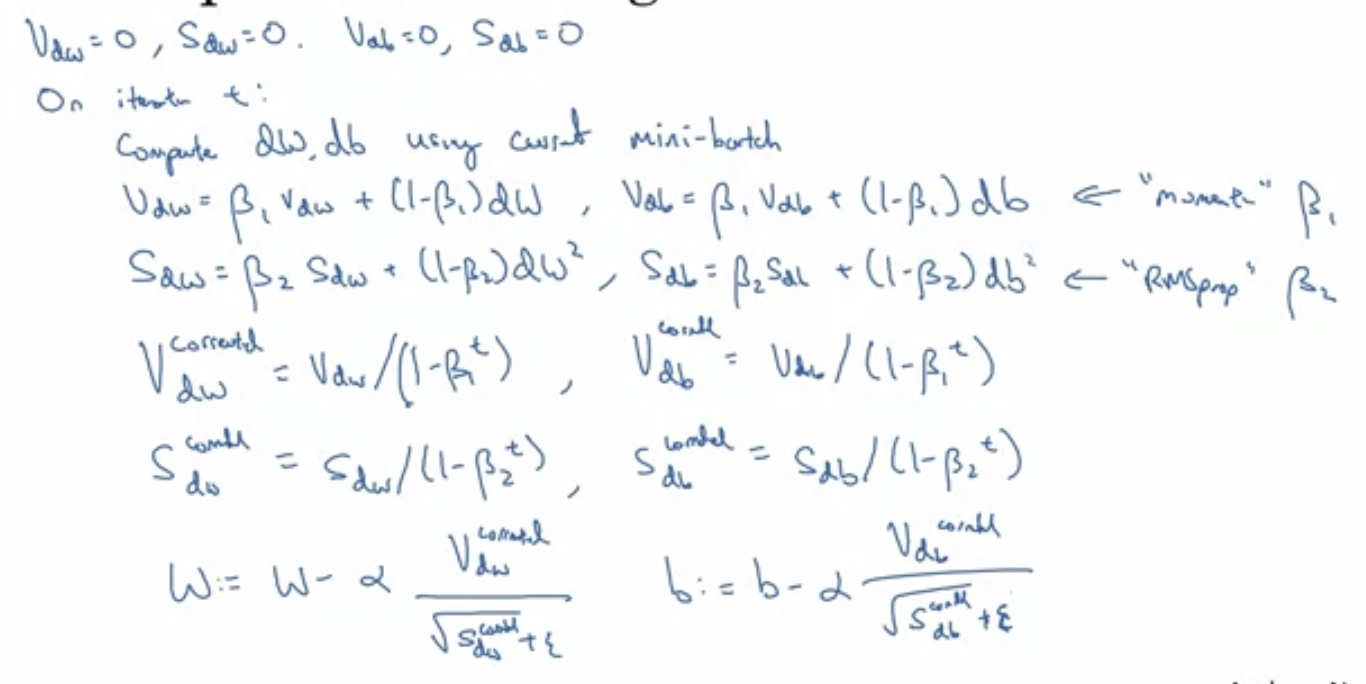
• Hyperparameters
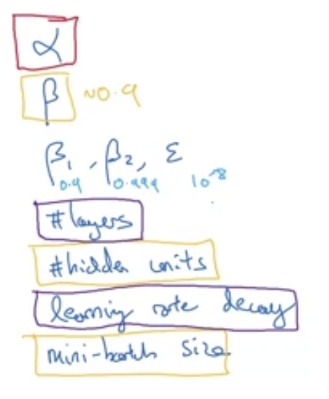
  • $\alpha$: try different values
  • $\beta_{1}$: try 0.9 first
  • $\beta_{2}$: try 0.999 first
  • $\varepsilon$: just use $10^{-8}$

• Basically, make $\alpha$ smaller over time.
• Fast when far from optimal –> Slow to be more precise and counter noise
• Formula:
  • $\alpha = \frac{1}{1 + rate \times epoch-num}$
  • or $\alpha = 0.95^{epoch-num}$
  • manual
  • things like that, as long as it decreases

• Intuition tells us that the training may get stuck as shown here:
  
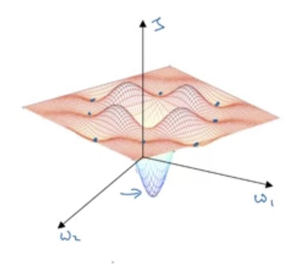
• However in higher dimensions, this is unlikely to happen because the derivative of every dimension has to be zero

Objective:

Explore TensorFlow, a deep learning framework that allows you to build neural networks quickly and easily, then train a neural network on a TensorFlow dataset.

• Order of importance (maybe) (red –> yellow –> purple –> not important):
  
• Good practice
  • Don’t use grid sampling where some hyperparameter is kept constant! Sample randomly helps to try out more values for every hyperparameter.
  • Zoom in to smaller range when a few value around the area are good (==> think render region)
• Use the appropriate scale
  • Uniform sampling can be inefficient
  • So, other scales are
    • log
      • example implementation:
        1. r = -4 * random.rand()
        2. alpha = 10**r
    • exponential
  • Think about the algorithm’s sensitivity to the hyperparameters
• Practical schools of thoughts
  1. Babysitting aka Panda: train, watch, and change hyperparameters along the way (use when no computational resource)
  2. Parallel aka Caviar: train many models at the same time

• Just like normalising input data set, normalising Z (or A) helps to speed up training
  • Well, here’s how to do it, whatever this is
    
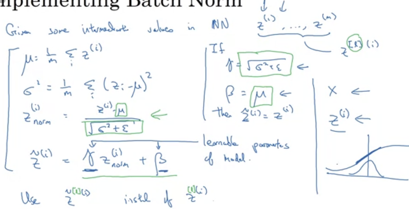
  • And the formula, whatever it is
    
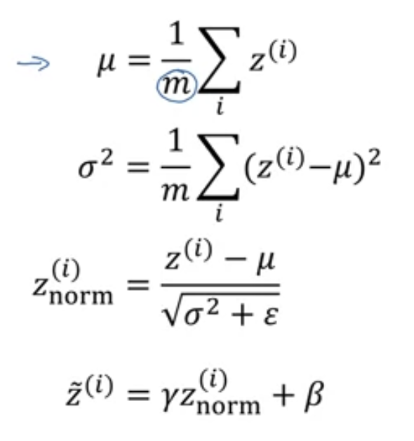
  • the beta here is another beta
  • beta and gamma are extra parameters and can be updated by gradient descent
  • when using bash normalisation, b becomes useless so it can be removed
• In a network, bash normalisation happens in between the computation for Z and A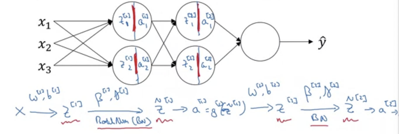
  
• Why it works
  • Covariate shift: without normalisation, hidden layers get inputs that change all the time. Making the input for a hidden layer to look more regular thus makes discovering the pattern easier for later layers.
  • Regularisation: it acts a bit like dropout because it introduces noise so later layers don’t depend too much on one unit on the previous unit. (Don’t use it as the regularisers though)
• When running test for one test case
  • When doing so, we don’t have a batch for the normalisation algorithm to do the normalisation
  • What we do instead is to do an exponentially weighted average for $\mu$ along with the $\gamma$ and $\beta$ learnt in the training process

• Why?
  • We use this when trying to recognise multiple classes^[softmax is actually a generalisation to logistic regression]
  • The number of classes is denoted by $C$
  • y_hat.shape = (C, 1)
  • Vecorisation: Y_hat.shape = (C, m)
• Softmax as a special activation function for layer [L]
  • Basically, we want to map the values of ZL to probabilities that sum to 1.
  • Formula $$a^{[L]}=\frac{e^{Z^{[L]}}}{\sum_{i=1}^{C} t_{i}}$$
• How to train?
  • We compare the sofmax to the hot max^[this is a vector with one 1 and 0 everywhere else that represents the correct y value]
  • Intuitively, we can use a loss function that minimises when the $\hat{y}$ for the class is as close to one as possible
  • Loss function: $$\mathcal{L}(\hat{y}, y)=-\sum_{j=1}^{4} y_{j} \log \hat{y}_{j}$$
  • Cost function: $$J\left(w^{[1]}, b^{[1]}, \ldots\right)=\frac{1}{m} \sum_{i=1}^{m} L\left(\hat{y}^{(i)}, y^{(i)}\right)$$
  • Back prop: $$\frac{\partial J}{\partial z^{[L]}} = \hat{y} - y$$

Tensorflow has a tape feature that can optimise parameters automatically based on a cost function (so there’s no need to write a backward prop)

Observe and figure out what this code does:

import numpy as np
import tensorflow as tf

w = tf.Variable(0, dtype=tf.float32)
x = np.array([1.0, -10.0, 25.0], dtype=np.float32)
optimizer = tf.keras.optimizers.Adam(0.1)

def training(x, w, optimizer):
	def cost_fn():
		return x[0]*w**2+x[1]*w+x[2] 
	for i in range(1000):
		optimizer.minimize (cost_fn, [w])
	return w

w = training(x, w, optimizer)
print(w)

The output:

<tf.Variable 'Variable:0' shape=() dtype=float32, numpy=5.000001>

DONE! :D