Neural Networks and Deep Learning
#course #computer-science #machine-learning #torefactor
This is the first course of the Coursera Deep Learning Specialisation by Andrew Ng.
H2 Course summary
According to the course description on Coursera:
If you want to break into cutting-edge AI, this course will help you do so. Deep learning engineers are highly sought after, and mastering deep learning will give you numerous new career opportunities. Deep learning is also a new “superpower” that will let you build AI systems that just weren’t possible a few years ago.
In this course, you will learn the foundations of deep learning. When you finish this class, you will:
- Understand the major technology trends driving Deep Learning
- Be able to build, train and apply fully connected deep neural networks
- Know how to implement efficient (vectorized) neural networks
- Understand the key parameters in a neural network’s architecture
This course also teaches you how Deep Learning actually works, rather than presenting only a cursory or surface-level description. So after completing it, you will be able to apply deep learning to a your own applications. If you are looking for a job in AI, after this course you will also be able to answer basic interview questions.
H2 Week 1 - Welcome and Introduction to Deep Learning
Objective:
Be able to explain the major trends driving the rise of deep learning, and understand where and how it is applied today.
H3 Significance of Deep Learning
- AI has been transforming many aspects of modern world
- Search engines
- Medicine
- Produce design
- Agriculture
- Transportation
- …
- “AI is the new Electricity”
- Cat recogniser is the tradition of learning deep learning
H3 What is a NN
- NNs takes inputs and produce some kind of prediction using a model
- A ReLU (Rectified Linear Unit) function takes on the value 0 for a wile and take off as a linear function
- Single neuron = linear regression without activation = preceptron
- When a machine learns, thy figure out what happens in between the input and the output
H3 Supervised Learning
- Supervised learning is when we try to fit a ML model to a desired output with a set of input is given
- Applications
- Real estate
- Online advertising
- Photo tagging
- Speech recognition
- Machine translation
- Autonomous driving
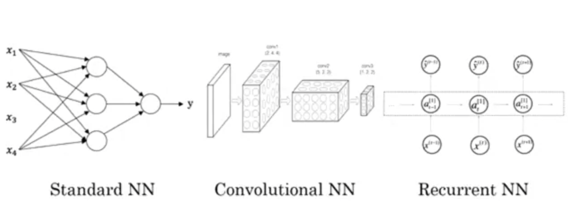
- Different types of supervised learning NNs
- CNN (convolutional NN), useful in computer vision
- RNN (recurrent NN), useful in speech or language processing that include sequenced data
- Standard NN
- Hybrid/custom
- Data structure
- Structured data: databases and tables
- Unstructured data: something like audio, image, text
H3 The Recent Rise of Deep Learning
- Deep learning is taking off for these three reasons:
- Data
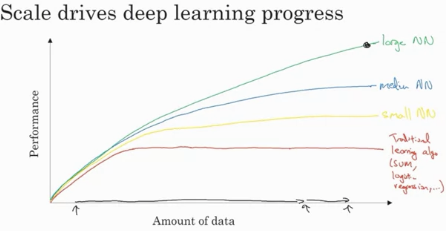
- Different NN architecture produces different performance curve based on the amount of labeled data (denoted by $m$ in this course) available
- Therefore, when we have enough data and scale, the performance increases
- According to the graph
- With small amount of data, it is unclear which NN scale is good
- With large amount of data, bigger NN is good
- Different NN architecture produces different performance curve based on the amount of labeled data (denoted by $m$ in this course) available
- Computation
- CPUs
- GPUs
- TPUs
- Distributed computing
- AISC (application-specific integrated circuit)
- M1
- Algorithm
- Using ReLU rather than Sigmoid made the algorithm run faster.
- This is because it eliminates the vanishing gradient problem.
- Data
- When we have improvement of all of these, the development of NN speeds up.
H3 Discussion Forum Rules
- Basically, do the right thing
- Don’t bully
- Don’t post inappropriate stuff
- Stay on topic
- Upvote thoughtful contents
- Avoid misunderstandings
- Cite ideas
- Provide as much information as possible when asking questions
- Don’t share your code
H2 Week 2 - Neural Networks Basics
Objective:
Learn to set up a machine learning problem with a neural network mindset. Learn to use vectorization to speed up your models.
H3 Binary Classification
- For loops are not encouraged
- Forward propagation and backward propagation is a common structure of a ML algorithm
- A binary image classification turns an image into a matrix containing all its pixel information and fits it into a model that outputs 0 or 1
H3 Notations
- A training example will be represented as $(x, y)$, where $x$ is a vector with $n_x$ elements and $y$ is either 1 or 0
- There are $m$ or M training examples. Sometimes $m_{\text{train}}$ and $m_{\text{test}}$ are used to differentiate different example types.
- Capital $X$ refers to all training examples combined:
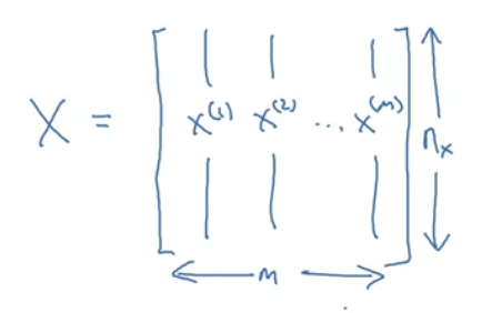
- Though implementing the matrix in the other direction also works, this version is more efficient
- Running
X.shapewill give $(n_x, m)$
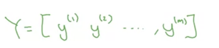
- It’s also convenient to combine all $y$s into $Y$, which looks like:
- Running
Y.shapewill give $(1, m)$
- Running
- The output of the logistic regression is $\hat{y} = P(y=1|x)$
- The weight of a layer will be $w$, it’s a $(n_x, 1)$ dimensional vector.
- The biases will be $b$, it’s just a number$
- The superscript $^{(i)}$ refers to the an individual training example
- In coding notation:
M is the number of training vectorsNx is the size of the input vectorNy is the size of the output vectorX(1) is the first input vectorY(1) is the first output vectorX = [x(1) x(2).. x(M)]Y = (y(1) y(2).. y(M))
H3 Logistic Regression
- Used when $y$ is either zero or one
- Since $\hat{y}$ is a probability between 0 and 1, a sigmoid function is applied before the output to squeeze the prediction to values between 0 and 1.
- The sigmoid function is defined to be $\sigma(z) = \frac{1}{1+e^{-z}}$, which makes this graph:
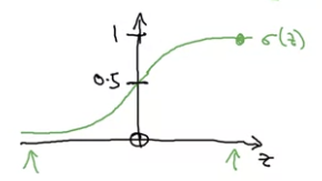
- The sigmoid function is defined to be $\sigma(z) = \frac{1}{1+e^{-z}}$, which makes this graph:
- The $\hat{y}$ output is thus computed using = $\hat{y} = \sigma(w^Tx+b)$
- The sigmoid function is a type of activation function
- Logistic regression is like a small neural network
H3 Cost Function
- The loss function $L(\hat{y}, y) = -(y\log{\hat{y}} + (1-y)\log{(1-\hat{y})})$ evaluates how well the algorithm is doing for one training example.
- A bit of intuition by substituting $y=1$ and $y=0$ demonstrates why this function make sense. When the actual data is close to 1, it wants $\hat{y}$ to also be close to one to minimise the loss.
- The cost function then tells the algorithm how well the weights and biases are doing on all training examples $$J(w, b)=\frac{1}{m} \sum_{i=1}^{m} L\left(\hat{y}^{(i)}, y^{(i)}\right)$$
H3 Gradient Descent
- The training process is essential trying to find the right $w$ and $b$ that minimises the cost.
- To be begin training, the values of $w$ and $b$ are initialised.
- How they are initialised doesn’t really for logistic regression because logistic cost is always concave down
- The descent process is done through multiple steps, during which $w$ and $b$ are updated according to a given learning rate just like:
Repeat { w := w - alpha * dJ(w, b)/dw b := b - alpha * dJ(w, b)/db } - In the computation graph, which shows the computation from left to right, gradient descent are the red parts in this picture
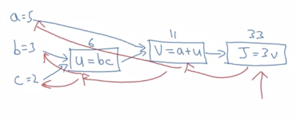
H3 Computing Derivatives
- The chain rule helps to compute how changing one thing affects other things like the output
- The most convenient method, then, is to start from the right and move to the left to find the derivatives.
- Most of the time, we ultimately want to find $\frac{d\text{ FinalOutput}}{d\text{ var}}$
- However, we don’t want to write all of that when coding, so the convention is writing
dvar.
H3 Implementation
- Implementation of loss function:
- (Computation graph is probably overkill for logistic regression)
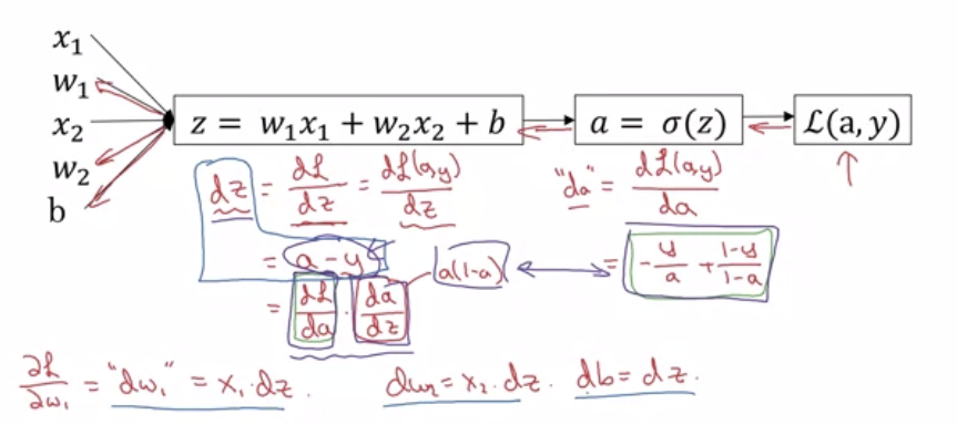
- Assuming that there are only two features
x1andx2, the forward propagation looks like:- The inputs are
x1w1x2w2andb - Then
z := w1 * x1 + w2 * x2 + b - Then
y_hat = a := sigmoid(z) - Then
loss := loss(a, y)
- The inputs are
- Moving backward:
- Take derivative of the sigmoid function and we get
da$\frac{d \hat{y}}{da} = - \frac{y}{a} + \frac{1-y}{1-a}$$ - Using the chain rule,
dzwould be $\frac{d \hat{y}}{dz} = a - y$; the derivation according to coursera forum:
Logistic regression dz derivation dw1would bex1 * dzdw2would bex2 * dzdbwould bedz
- Take derivative of the sigmoid function and we get
- The full derivation
- Implementation of cost function given m examples and changing the parameters accordingly
- Recall the formula for cost function: $$J(w, b)=\frac{1}{m} \sum_{i=1}^{m} L\left(\hat{y}^{(i)}, y^{(i)}\right)$$
- Doing some fancy math, it turns out that the overall derivatives across the whole training set can be obtained by simply averaging the derivatives for every single training example.
- So, the algorithm would be
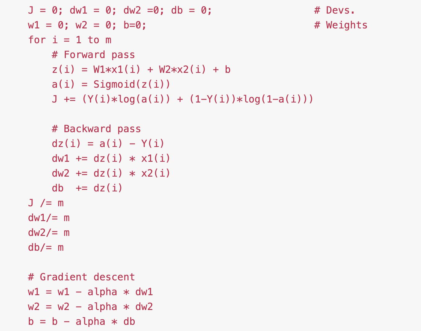
- A human readable breakdown of what this algorithm does
- Initialise
Jdw1dw2dband use them as accumulators - Repeat for all training examples:
- forward propagation
- Add loss to the cost accumulator
- find
dzand thencedw1dw2dbof the single training example and add it to the accumulator
- Find average value of
J, that’s the correct cost - Find average value of
dw1dw2db - Change
w1w2bby the derivative weighted by the learning ratealpha
- Initialise
- Note that this code should run for multiple iterations to minimise error
- However the weakness of this algorithm is that you have to write two
forloops and that’s not good. Course 1 - Neural Networks and Deep Learning of the for loop can make the code more efficient.
- A human readable breakdown of what this algorithm does
H3 Vectorisation
- Vectorisation helps to implement the learning algorithm without explicit
forloops. This will make the programme run more efficiently because vector calculations are usually very well-optimised in python libraries like NumPy- And we can make use of GPUs
- Wondering if there’s a way to use the M1 neural engine
- This allows us to process large data sets quickly
- Note: to implement, first do
import numpy as npto import NumPy. Here are some usefully NumPy methods that are vectorised for vector $v$:np.log(v)to take lognp.exp(v)to raise $e$ to the power of values in that vectornp.abs(v)np.maximumfind maximumv**2square itnp.sum(v)gives the sum of the tings in that vector
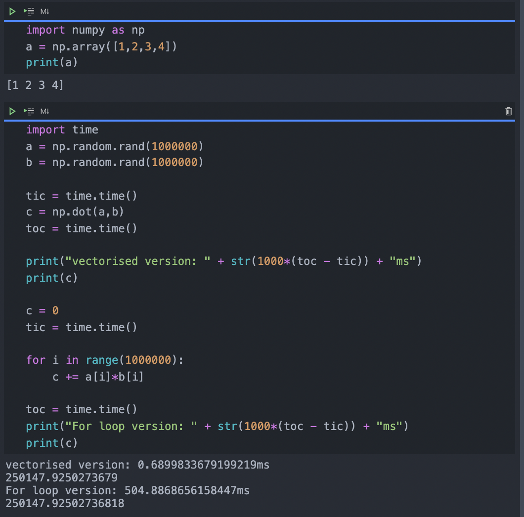
- An example of vectorisation
- Both algorithm in this screenshot produce the same result, but the vectorised version is almost 1000 times faster
- Both algorithm in this screenshot produce the same result, but the vectorised version is almost 1000 times faster
- Implementations
- Single training example implementation
- Basically, we replace all the
dw1dw2… with one single vectordw - The new
dwis initialised to be all zeros usingnp.zeros((n_x, 1)) - Instead of
dw1 += x1[i]dz1[i]and so on, we just usedw += x[i]dz[i] dw1 = dw1/mand so on becomesdw/=m
- Basically, we replace all the
- Whole training set implementation
Xstacks together allxs and has the shape(n_x, m)zwill thus allzs stacked in a rowbwill also have allbs stacked in a rowztherefore= np.dot(w.T X) + bAis allas stacked in a row- There will also be a vectorised version of
sigmoid()
- Gradient computation implementation
Z = np.dot(w.T, X) + bdZis alldzs stacked horizontally, i.e.(1, m)matrixdZ = A - Y- `db = (1/m)(np.sum(dZ))
- `dw = (1/m)(np.dot(X, dz.T))
- Single training example implementation
- Broadcasting
- Broadcasting makes coding more flexible, but can also lead to strange bugs if not careful
- NumPy automatically stretch out a number or vector to fit the shape needed if possible to fit the operation
- To sum a matrix vertically, do
summed-vector = v.sum(axis=0)ornp.sum(v, axis = 0, keepdims = True) - To sum a matrix horizontally, do
summed-vector = v.sum(axis=1)ornp.sum(v, axis = 1, keepdims = True) - When adding number to vector, NumPy expands the number to the shape of the vector
H2 Week 3 - Shallow Neural Networks
Objective:
Learn to build a neural network with one hidden layer, using forward propagation and back propagation.
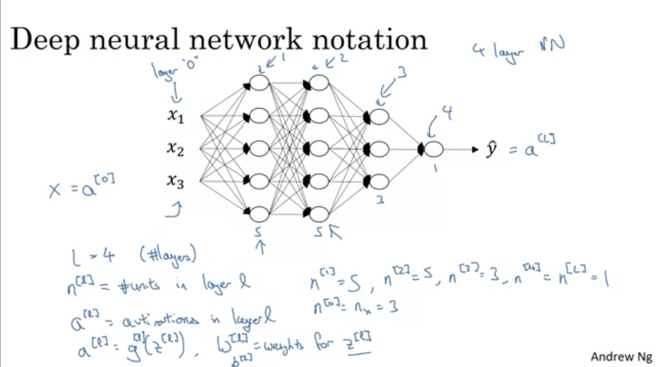
H3 More notations and definitions
- The superscript $^{[i]}$ refers to quantities associated with a layer
- For example, $W^{[1]}$ refers to the weights in the first hidden layer
- Layers
- The leftmost layer is called the input layer
- The rightmost layer is the output layer
- All layers in the middle are the hidden layers
- We don’t count the input layer in the NN layer count
H3 The architecture
- basically we stack together layers of logistic regression neurons
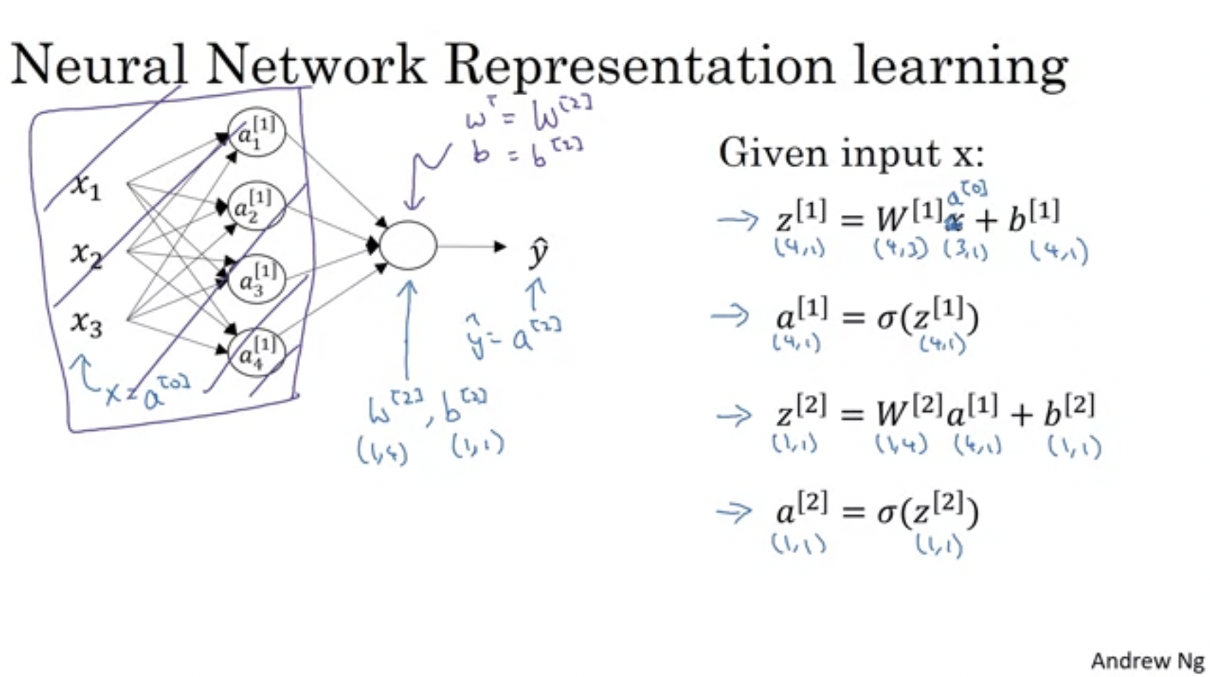
- Each neutron in each layer will simply do
activation_func(dot(w.T, x) + b) - But we always want to vectorised the network like so
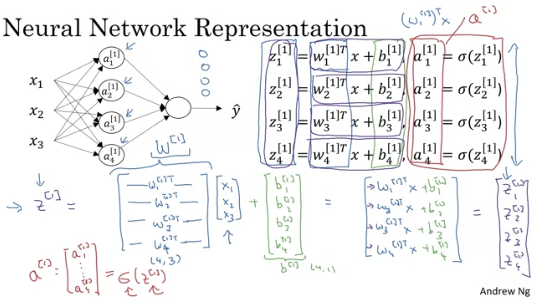
- The matrix dimensions in this case is… but we can always go in and figure this out
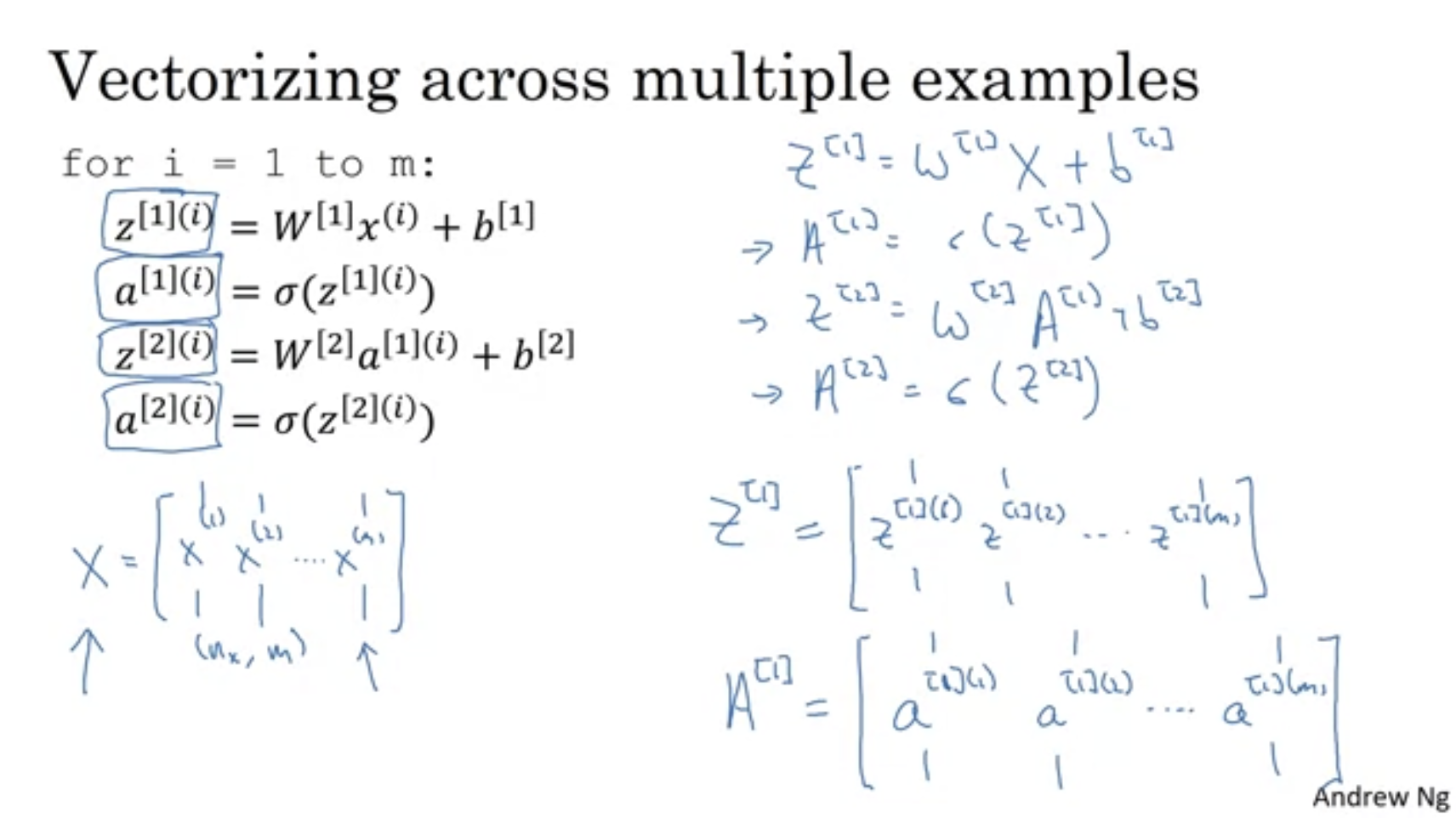
- Taking it further, it can be vectorised for multiple training examples like this
H3 Activation functions
- There are different activation functions that we can use, and choosing which one to use does affect performance
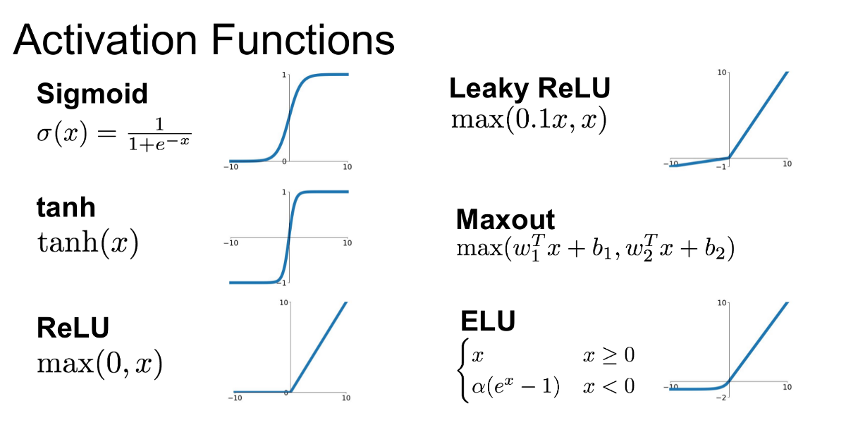
- Which one to use
- Usually use ReLU by default
- Leaky ReLU is good as well
- Never use sigmoid unless it’s the final layer for binary classification
- Just try them out!
- Wait, but why not just use linear?
- Because it turns out that if we do this, the whole network is just going to calculate y as a linear function of x. No point right?
- So use this unless you want the output to be all real number
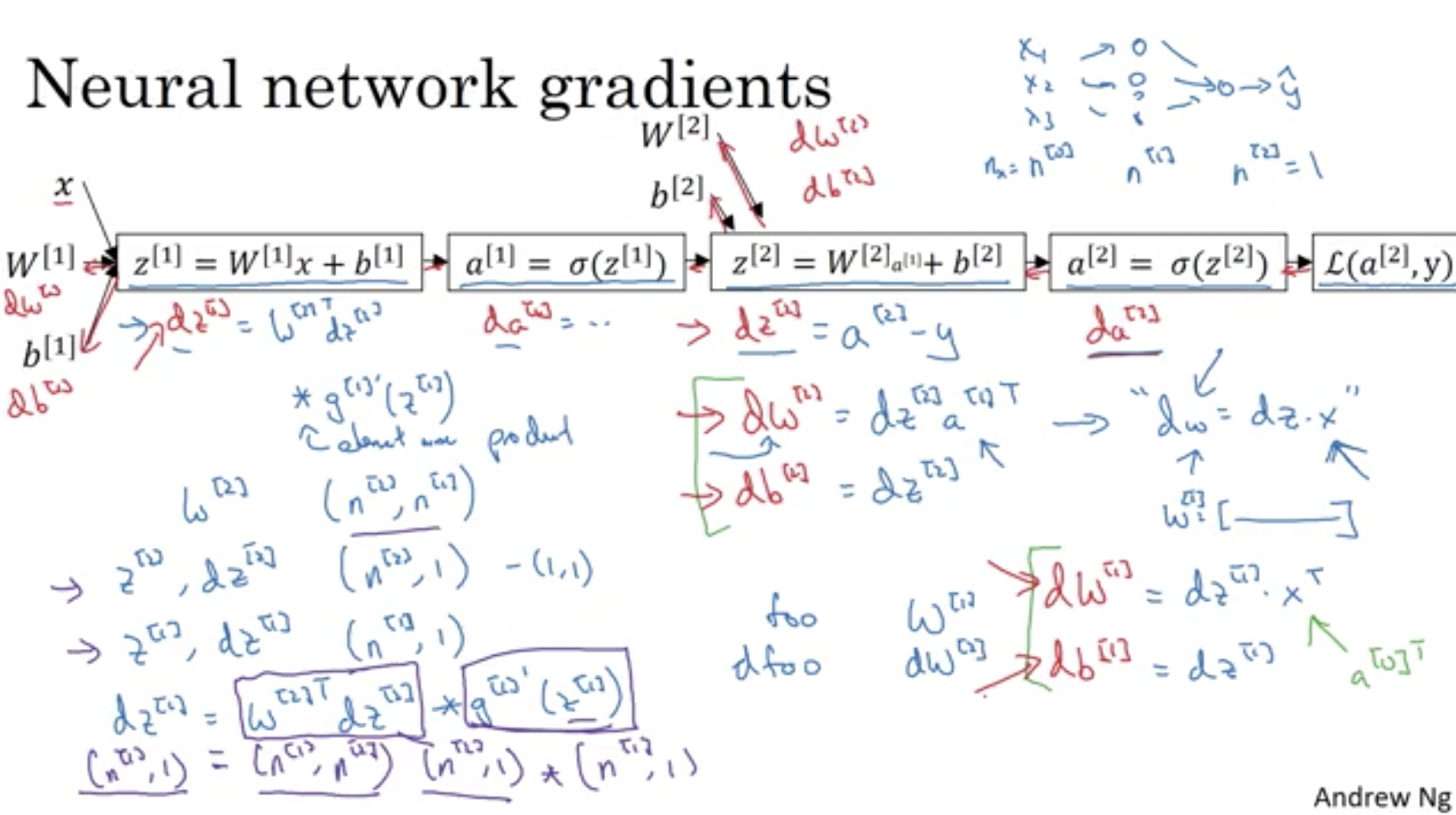
H3 Gradient descent for NN
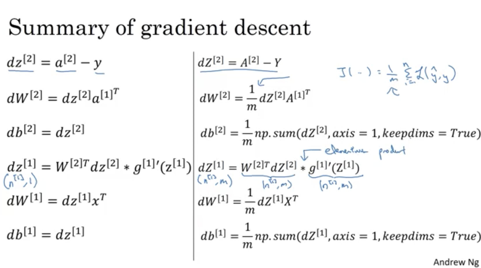
- Do the math. If everything done correctly, the resultant equations should be:
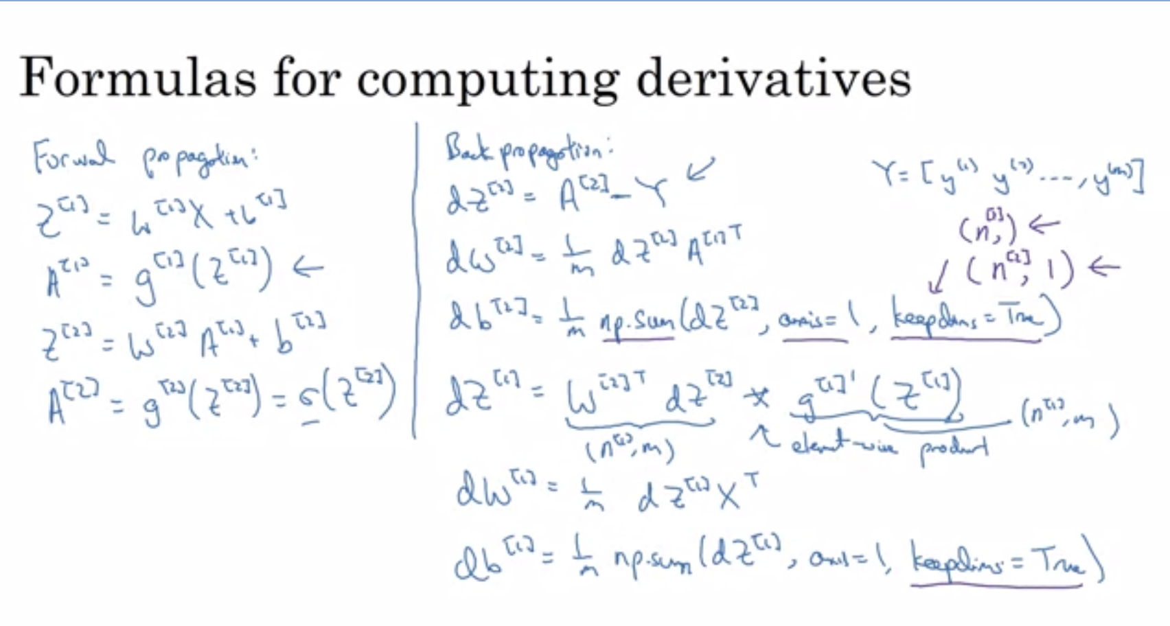
- If confused, the derivation looks like
- Vectorising gives
H3 The algorithm
- Initialise the parameters randomly this time
- Why? Because if we do that, the neurons in the hidden layers are going have identical parameters (aka symmetrical) and will thus compute the exact same thing no matter how you train them.
- To initialise a layer, use the numpy function
W1 = np.random.randn((2,2)) * 0.01- We usually want to initialise the values to small numbers so that we end up on the ‘high contrast’ part of the activation function; that’s what the
* 0.01is for
- We usually want to initialise the values to small numbers so that we end up on the ‘high contrast’ part of the activation function; that’s what the
- The exception is the values of b which can be initialised to all be zeros using `b1 = np.zero((2,1))
- Forward prop
Z1 = W1A0 + b1    # shape of Z1 (noOfHiddenNeurons,m)
A1 = sigmoid(Z1)  # shape of A1 (noOfHiddenNeurons,m)
Z2 = W2A1 + b2    # shape of Z2 is (1,m)
A2 = sigmoid(Z2)  # shape of A2 is (1,m)
The mathematical write out for one example $x^{(i)}$: $$z^{[1] (i)} = W^{[1]} x^{(i)} + b^{[1]}\tag{1}$$ $$a^{[1] (i)} = \tanh(z^{[1] (i)})\tag{2}$$ $$z^{[2] (i)} = W^{[2]} a^{[1] (i)} + b^{[2]}\tag{3}$$ $$\hat{y}^{(i)} = a^{[2] (i)} = \sigma(z^{ [2] (i)})\tag{4}$$ $$y^{(i)}_{prediction} = \begin{cases} 1 & \mbox{if } a^{[2](i)} > 0.5 \\\ 0 & \mbox{otherwise } \end{cases}\tag{5}$$ Combining the examples $J$ can thus be computed using: $$J = - \frac{1}{m} \sum\limits_{i = 0}^{m} \large\left(\small y^{(i)}\log\left(a^{[2] (i)}\right) + (1-y^{(i)})\log\left(1- a^{[2] (i)}\right) \large \right) \small \tag{6}$$ - Backward prop
dZ2 = A2 - Y      # derivative of cost function we used * derivative of the sigmoid function
dW2 = (dZ2 * A1.T) / m
db2 = Sum(dZ2) / m
dZ1 = (W2.T * dZ2) * g'1(Z1)  # element wise product (*)
dW1 = (dZ1 * A0.T) / m   # A0 = X
db1 = Sum(dZ1) / m
# Hint there are transposes with multiplication because to keep dimensions correct
H2 Week 4 - Deep Neural Networks
Basically, we are putting everything together
Objective:
Understand the key computations underlying deep learning, use them to build and train deep neural networks, and apply it to computer vision.
H3 L-layers neural network
- Shallow NN is a NN with one or two layers.
- Deep NN is a NN with three or more layers.
- Sometimes deeper networks allow you to solve complicated problems
- You don’t always know how many layers to use
- Refer to this for notation conventions.
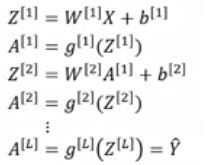
H3 Forward propagation
- Do the same recurring weighting-biasing-activation calculation for each layer
- The unvectorised version would look like
z[l] = W[l]a[l-1] + b[l] a[l] = g[l](a[l]) - Vectorising the process yields:
Z[l] = W[l]A[l-1] + B[l] A[l] = g[l](A[l]) - We need a for loop to forward propagation for all layers. We can’t really vectorise this but it’s okay
H3 Matrix dimensions
- Pen and paper is usually good for debugging matrix dimensions
- Don’t take the following as granted. Mathematical intuition brings you to:
- Dimension of
Wis(n[l],n[l-1]) - Dimension of
bis(n[l],1) dwhas the same shape asW, whiledbis the same shape asb- Dimension of
Z[l],A[l],dZ[l], anddA[l]is(n[l],m)
- Dimension of
H3 Why go deep
- There are multiple theories
- Feature detection
- ==> refer to 3b1b playlist
- Circuit theory
- Simplifically: increasing network layer count will somehow require the units count to increase exponentially to solve the same problem
- Or, $O(\log{n})$
- For example:
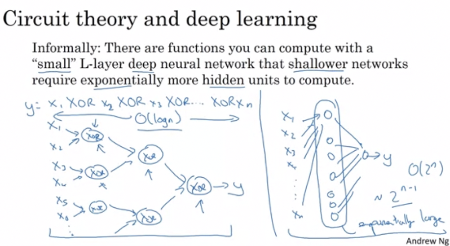
- “Deep” is just a fancy word for branding
- Feature detection
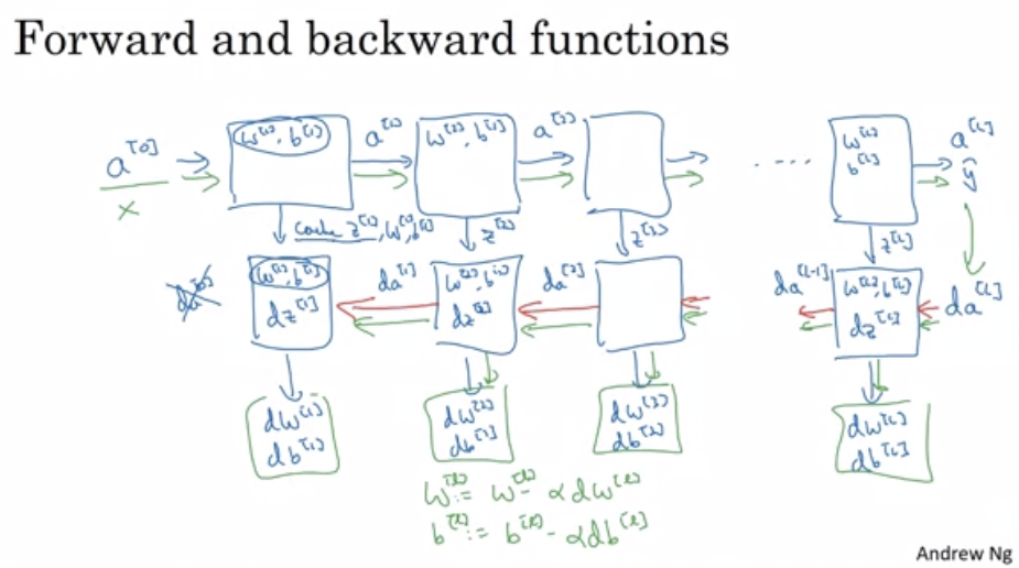
H3 Building a deep NN
- We usually cache some results for each layer to save time for back prop
- Forward and backward propagation for a layer
l: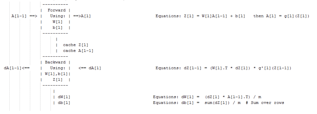
- Note that we usually cache some results for each layer to save time for back prop
- Math for forward prop
- Code for forward prop will do something like this
Input A[l-1] Z[l] = W[l]A[l-1] + b[l] A[l] = g[l](Z[l]) Output A[l], cache(Z[l]) - Math for backward prop:
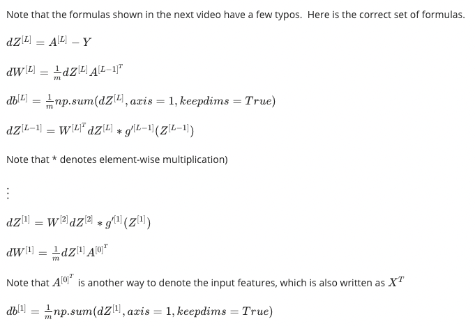
- Code for backward prop will do something like this
Input da[l], Caches dZ[l] = dA[l] * g'[l](Z[l]) dW[l] = (dZ[l]A[l-1].T) / m db[l] = sum(dZ[l])/m # Dont forget axis=1, keepdims=True dA[l-1] = w[l].T * dZ[l] # The multiplication here are a dot product. Output dA[l-1], dW[l], db[l] - The derivative for the final layer with respect to the loss function is
dA[L] = (-(y/a) + ((1-y)/(1-a)))
- Stacking layers together gives
- Probably use ReLU for hidden layers
H3 Parameters vs Hyperparameters
- Parameters are your
Ws andbs that determine how to get from data to output - Hyperparameters are other things that affect how the NN behave, including:
- Learning rate alpha
- Number of iterations
- Number of hidden layers L
- Number of hidden units
- Activation functions
- …
- Trying out hyperparameter values and comparing the results is a good way to optimise hyperparameters.
- There is a systematic way to try out hyperparameters
- Optimal hyperparameters can change over time
H3 Something to do with the brain?
- Not much.
- Might have something to do with brain neurons firing, but really, neuron scientist havn’t figured out how they work yet
done :D